Dez 2018

A curious measurement

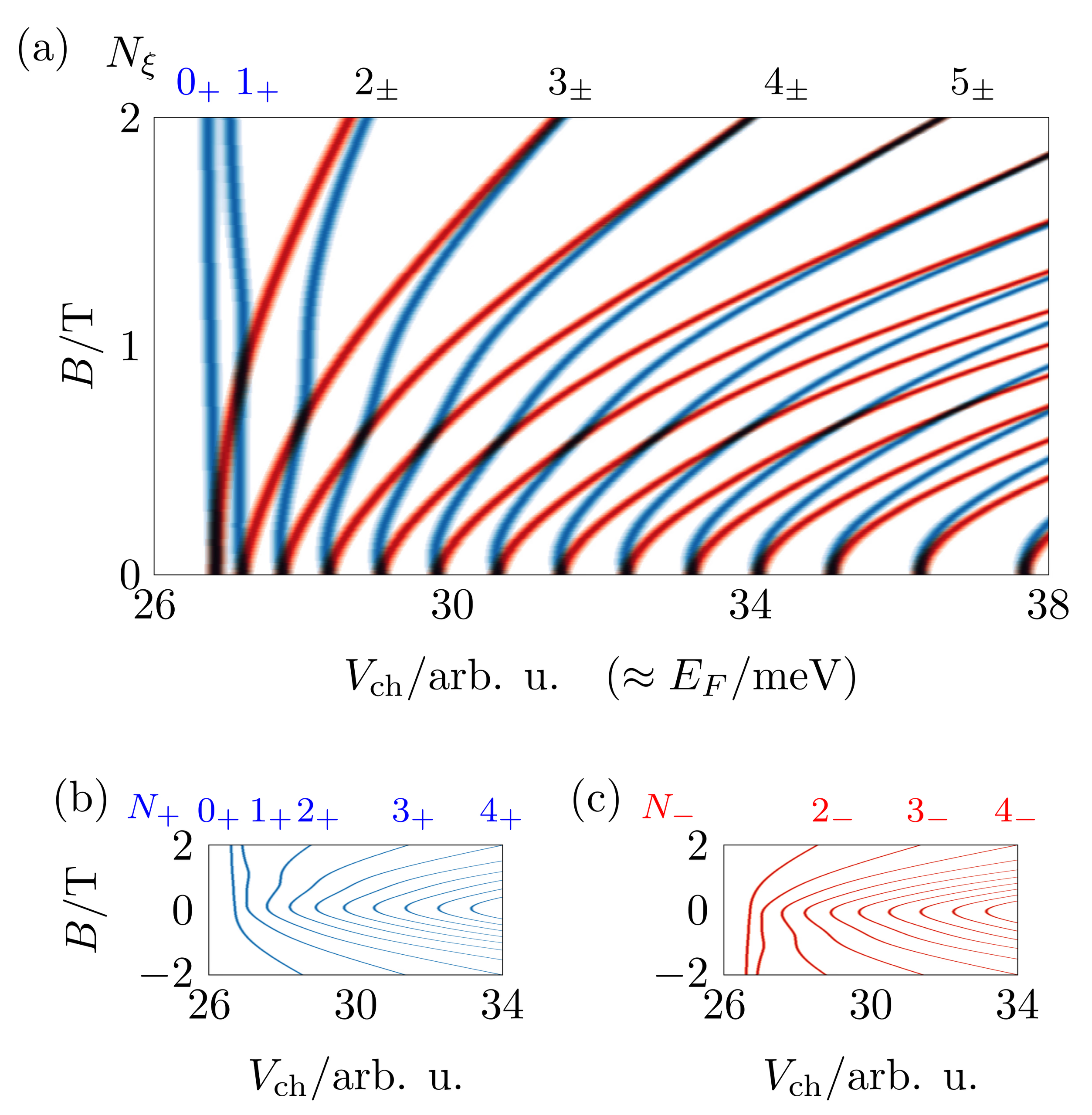
At the Kirchberg conference, the experimentalists from ETH Zürich came to us with transconductance measurements of electrostatically defined quantum point contacts in bilayer graphene. The fan diagrams showed a striking interweaving pattern: fourfold (spin+valley) degenerate modes at zero magnetic field split into twofold (by valley) at intermediate fields, then restore fourfold degeneracy in the quantum Hall regime. During that transition, levels from one valley shift by exactly two in quantum number relative to the other. The pattern was robust across different QPCs, channel widths, and displacement fields. Why? Or was the "two" a coincidence?

Numerical Calculation

We could quickly reproduce the pattern numerically by sweeping the magnetic field in a tight-binding eigenvalue computation of the states in the ribbon. The two limiting cases are even solvable by hand: At $B = 0$ we have valley degenerate size-quantized modes and at high $B$ we see Landau levels.

The answer is already visible in the effective low-energy Hamiltonian of bilayer graphene. In a perpendicular magnetic field it reads

where $\lambda_B = \sqrt{\hbar c/(eB)}$ is the magnetic length, $m = \gamma_1/(2v^2)$, and $\xi = \pm 1$ is the valley index. The key object is the operator $\pi = \tilde{y} + ip_{\tilde{y}}$, which in a magnetic field becomes proportional to the harmonic oscillator lowering operator $a$. The off-diagonal blocks contain $\pi^2$ — this squared structure, specific to bilayer graphene, is a winding number $J = 2$.

What are the zero-energy eigenstates of this Hamiltonian? They must satisfy $\pi^2|\psi\rangle = 0$, i.e., $a^2|\psi\rangle = 0$. There are exactly two such states — the harmonic oscillator ground state $\phi_0$ and first excited state $\phi_1$. These two zero modes live entirely on one sublattice. When a displacement field is applied, that sublattice polarization pins them to one layer, and they appear only in one valley's conduction band (say $K_+$ for $B > 0$). All higher Landau levels $N \geq 2$ appear in both valleys.

This asymmetry dictates what must happen during the adiabatic transition from zero field to high field. At $B = 0$, both valleys have the same size-quantized states: $n = 1, 2, 3, \ldots$ At high $B$, valley $K_+$ has Landau levels $N = 0, 1, 2, 3, \ldots$ in the conduction band, while $K_-$ has only $N = 2, 3, 4, \ldots$ — it is missing two states. Since the evolution is smooth and levels cannot appear or disappear, the only consistent mapping is that $K_-$ levels must shift up by two: the size-quantized state $n_{K_-}$ evolves into Landau level $(n+2)_{K_-}$. This is the interweaving pattern we observe.

Topological Invariants

This is actually an index theorem at work. The number "two" is the index of the operator $\pi^2$. In general, the index of an operator $D$ is defined as

— the number of zero modes of $D$ minus the number of zero modes of $D^\dagger$. For our operator $\pi^2$: the kernel has dimension two (the states $\phi_0, \phi_1$), while the kernel of $(\pi^\dagger)^2$ is empty (there are no normalizable solutions). So $\mathrm{ind}(\pi^2) = 2$.

The index cannot change under continuous deformations of the operator. So changing the channel width, the displacement field, the shape of the confinement potential - these don't appear in $\pi$.

The adiabatic transition between the two regimes is an instance of spectral flow: as the magnetic field is turned on, eigenvalues move continuously, and the net number of states that "flow" from one part of the spectrum to another is fixed by the index. The spectral flow equals the index equals the winding number.

Generalization

This was all a single-valley calculation. The full lattice Hamiltonian contains both $K_+$ and $K_-$ with opposite winding ($+2$ and $-2$), and the total index is zero — as guaranteed by the Nielsen-Ninomiya theorem. So why do we observe the clean single-valley topology and not a mix? Because inter-valley scattering requires momentum transfer on the order of the inverse lattice constant.

The generalization is: For monolayer graphene the Hamiltonian has $\pi^1$ in the off-diagonal — winding $J = 1$. There is one zero mode, and the shift between valleys during the adiabatic transition is one. While the smooth confinement for single-layer graphene is hard to achieve experimentally, we confirmed this numerically. For ABC-stacked trilayer graphene, $J = 3$, the prediction is three zero modes and a shift by three.

Read the paper Topologically nontrivial valley states in bilayer graphene quantum point contacts by Hiske Overweg, Angelika Knothe, Thomas Fabian, Lukas Linhart, Peter Rickhaus, Lucien Wernli, Kenji Watanabe, Takashi Taniguchi, David Sánchez, Joachim Burgdörfer, Florian Libisch, Vladimir I Fal’ko, Klaus Ensslin, Thomas Ihn; Phys. Rev. Lett. 121, 257702 (2018) here or on arxiv.

← Blog