Okt 2022

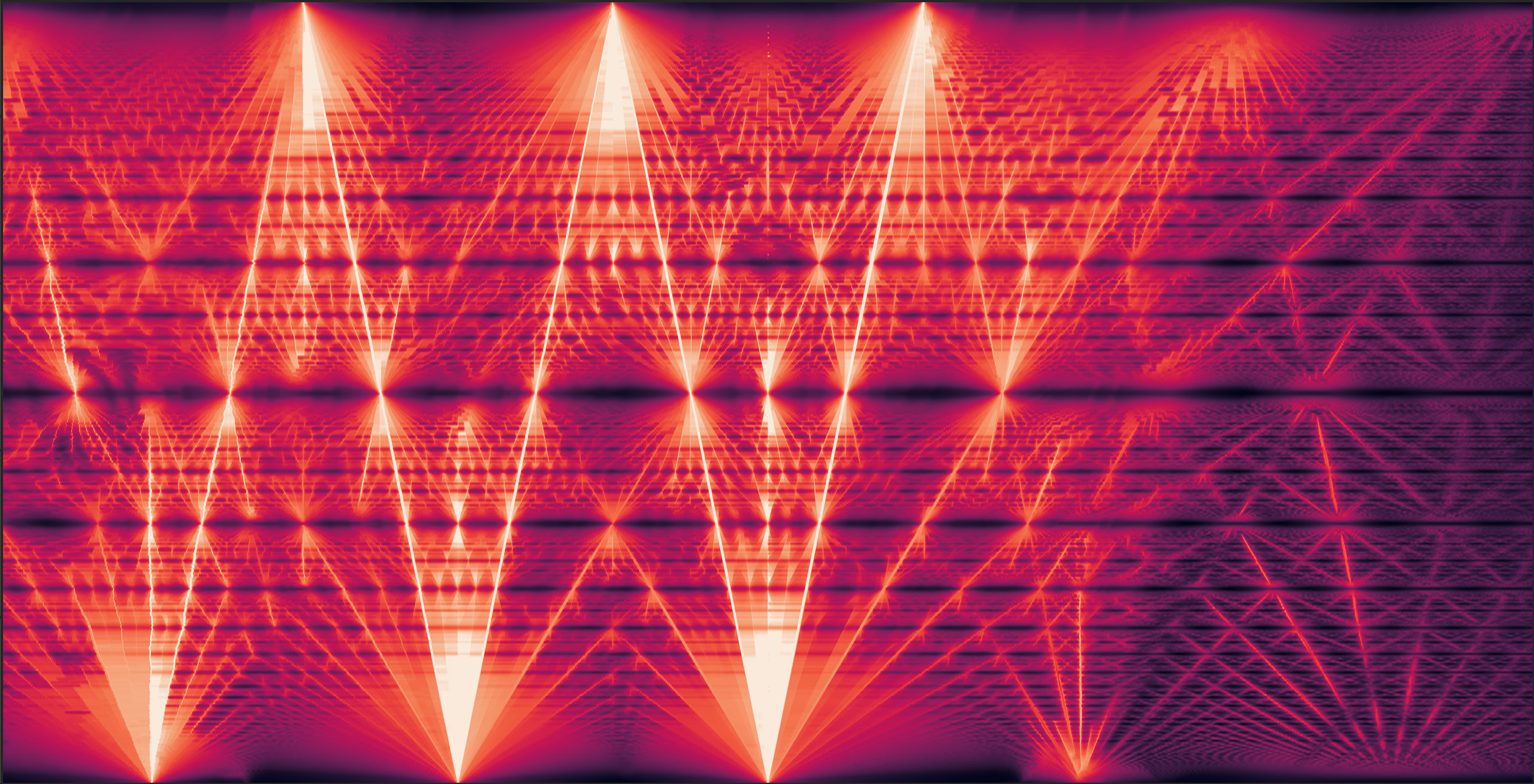
Hofstadter's butterfly in graphene

Electrons on a crystal lattice in a magnetic field produce a fractal energy spectrum. The allowed energies split, and split again, forming an infinitely self-similar pattern as the field strength varies. Douglas Hofstadter computed this in 1976 and it has been called Hofstadter's butterfly ever since.

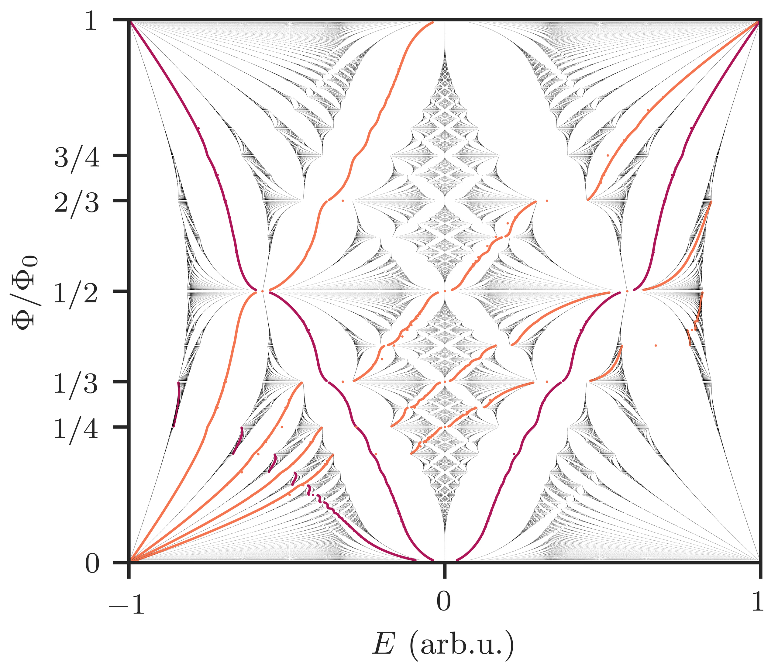
The fractal structure emerges on any periodic lattice, but the specific pattern depends on the geometry. The one shown here is the butterfly of the honeycomb — graphene's lattice.

From eigenvalues to conductance

The butterfly shows energy eigenstates. Experiments, however, measure conductance — how well electrons flow through the material — and control the number of charge carriers via a gate voltage. To connect the fractal to a measurement, two transformations are needed.

First, we replace eigenvalues by conductance: at each energy and magnetic field, we compute how many quantum channels are available for transport. Regions dense with states carry large conductance. Gaps between groups of allowed energy levels — Landau levels — appear with low conductance. The butterfly remains recognizable, but now encodes where current flows and where it does not.

Second, we transform the vertical axis from energy to charge carrier density — obtained by counting the filled states below a given energy. This straightens the fractal. Gaps, which curve in the energy picture, become straight lines in the density picture. Their slopes and intercepts follow a simple linear relation, called the Wannier equation.

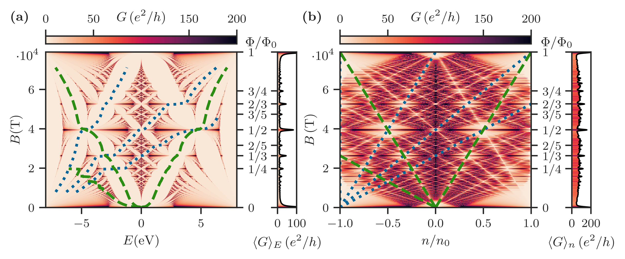
The Wannier equation states that the carrier density at which a gap appears is a linear function of the magnetic field, with integer coefficients. The slope encodes the Hall conductance of that gap; the intercept counts filled bands at zero field.

The moiré makes it real

Hofstadter's butterfly was long a theoretical amusement: a metal's unit cell is tiny. Threading a single magnetic flux quantum through it requires a magnetic field that is orders of magnitude beyond anything achievable in a lab.

That changed when graphene is stacked on hexagonal boron nitride. Since these two atoms are right next to each other in the periodic table, the two lattices are nearly but not perfectly matched, one is ever so slightly larger. When these materials are put on top of each other, there are regions where the atoms are right above each other, and regions where they are "between" each other, creating a so-called moiré pattern. The graphene atoms slightly deform due to this, and this deformation is itself a lattice. One magnetic flux quantum through this supercell corresponds to a field that can be reached in a lab.

Then the entire Wannier diagram — its linear gap structure, its conductance peaks at rational flux — becomes directly accessible in experiment.

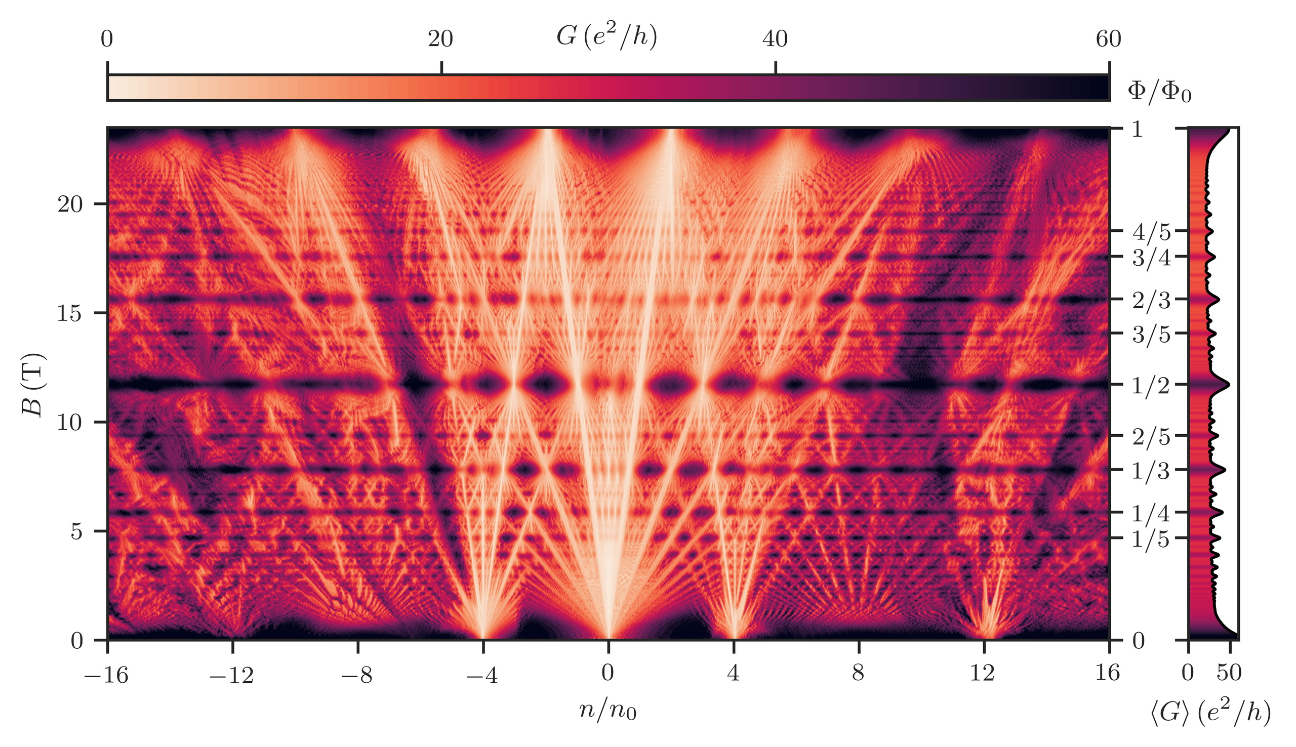
We computed this diagram from a tight-binding model of the full moiré supercell. The result agrees quantitatively with recent transport measurements.

Brown-Zak oscillations

The Wannier diagram shows two kinds of structure: tilted lines of low conductance (the gaps) and horizontal "color changes" of high conductance. The horizontal lines are Brown-Zak oscillations. At these special magnetic field values, translational symmetry is restored: After the electron has gone a number of unit cells further, it has "turned around" once. The electrons acquire a well-defined crystal momentum — they propagate as if the magnetic field were absent and the conductance peaks.

Notes for the experts

Computing conductance from the band structure

Computing the conductance for the full moiré supercell posed a challenge: the unit cell contains roughly 800,000 atomic sites. Standard quantum transport formalisms require matrix inversion at a cost that scales as $N^3$ — not feasible at this size. But, we found a trick: For a periodic system, the conductance is proportional to the number of propagating modes at a given energy, This number can be extracted directly from the band structure: each band contributes proportionally to its group velocity,

This eigenvalue problem requires only matrix factorization — not inversion — reducing the computational cost by orders of magnitude and making the full moiré calculation tractable.

Wannier equation for graphene

The linear dispersion of graphene modifies the Wannier equation to a half-integer form:

with degeneracy $g = 4$ (spin and valley). This is the same shift responsible for graphene's half-integer quantum Hall effect $\sigma_{xy} = 4(t+1/2)\, e^2/h$. Near the Dirac point, only the half-integer subset of gaps appears. Near the band edges, where the dispersion becomes parabolic, the full integer set is recovered. The satellite Dirac cones in the moiré system are spaced by $4\, n/n_0$ while the minimum slope from the half-integer equation is 2, breaking the periodicity in $\Phi_0$ — a feature clearly visible in experiment.

Read the paper: T Fabian, M Kausel, L Linhart, J Burgdörfer, F Libisch, "Half-integer Wannier diagram and Brown-Zak fermions of graphene on hexagonal boron nitride", Physical Review B 106 (16), 165412 here or on arxiv.

← Blog